A Guide to Contrast Enhancement: Transformation Functions, Histogram Sliding, Contrast Stretching and Histogram Equalization Methods with Implementations from Scratch using OpenCV Python

1.Introduction

Contrast enhancement is an important concept of image processing. It is widely used in image manipulation applications for decades. The word “contrast” specifies the difference between the pixel with the highest intensity value and the pixel with the lowest intensity value within an image. The contrast enhancement techniques aim to handle the common contrast issues. Thus, it tries to make image visually more aesthetic after appropriate operations. So we can interpret the image better than we understand before. It is also important in the field of computer vision and usually it is the first step as a preprocessing technique for most of the studies.

2.Prerequisites

Before getting started:

• You need to have Python 3 or higher version installed
• Using the command line or terminal, install the NumPy, OpenCV and matplotlib using the following commands with PIP if you don’t have:

pip install numpy
pip install opencv-python
pip install matplotlib

3.Subjects and Benefits

Subjects:

• Transformation functions: Log Transform, Exponential Transform, Power-law Transform
• Histogram Sliding
• Contrast Stretching(also known as Histogram Stretching)
• Histogram Equalization and Some of the State-of-art Methods:Classical Histogram Equalization, Brigthness Preserving Bi-histogram Equalization(BBHE), Equal Area Dualistic Sub-Image Histogram Equalization(DSIHE)

After reading this article, you will be able to:

• Describe and implement transformation functions, histogram sliding, contrast stretching and histogram equalization.
• Plot the images and their histograms.
• Enhance the contrast of gray and RGB(or color) images

4.Utility Functions

While you are reading the sections below, you will see some functions for essential operations like plotting, colorspace conversion etc. You can read this section now or return when you struggle during reading the article. I have created a script named “imutil.py” to avoid the code repetition and provide modularity. I also created and packed all the functions in one file named as “contutil.py” and I will explain each of these functions in order. The third file is “test_main.py” which is used to see the results and to test the functions. I inserted the link at end of the article if you would like to clone it on GitHub.

correct_gray(): OpenCV may not know the image we read from file is grayscale or not, if it is a single channel gray image, OpenCV treats it like a 3 channel image and all channels are equal to each other. One channel is enough and suitable for processing a gray image so I have coded this function.

bgr2gray(): This function converts and RGB image to gray using classical RGB to gray formula. The red channel is multiplied by 0.1140, the green channel is multiplied by 0.5870 and the blue channel is multiplied by 0.2989. We can use the below formula:

is_gray(): Since RGB images consist of 3 channels and gray images have single channel, we can check whether our image is gray or not. Moreover, if it is gray but has 3 channel due to treat of OpenCV to this image, if these 3 channels contain same values we can conclude that it is a gray image.

bgr2rgb(): OpenCV always uses BGR channel order and this situation causes matplotlib to plot distorted image. So before we plot the image, we have to make it to use RGB order.

rgb2ycbcr(): In earlier times, to equalize the histogram of the RGB images, researchers were applying histogram equalization to the R, G and B channels separately. Later it is found that it may not be appropriate, since the interest of histogram equalization is intensity and RGB histogram equalization may cause color distortion. We can convert our image to another colorspace like HSV, LAB, YUV or YCbCr to get the intensity channel(V, L, Y and Y respectively). You can also try other colorspaces especially for higher bit depth. To convert RGB to YCbCr, we can apply the formula below:

rgb2rgb(): Converts an YCrCb image back to RGB image, with the formula below:

im_plot(): Plots the images together in a figure and shows.

hist_plot(): Plots the histogram of the images together in a figure and shows. For RGB images, it shows the RGB histogram. For gray images, it shows graylevel histogram.

get_depth(): Gets the number of levels in an image.

5. Create or Download the Files

For the purpose of testing, you have to create the main function below:

Also, create files named “imutil.py” (which is given in Section 4) and “contutil.py” respectively. These files will be used to perform various operations. You can uncomment/comment the code lines in the main function to test utility functions. If you do not want to download “contutil.py”, create it and add these lines to start:

import cv2
from matplotlib import pyplot as plt
import math
import numpy as np
import imutil

Alternatively, you can download the test images and codes from the GitHub repository link:

EmreCanKURAN/ContrastEnhancementPack

6.Transformation Functions

We can accept an input image as a function of F(x, y) and output image as a function of G(x, y), which is processed. We can define a procesed point(or pixel) as in the Equation (1):

Equation (1)

In Equation (1), s is the processed pixel, T is the transformation function and r is the actual pixel that we are interested in. Transformation functions can vary and you may also come across different transformation functions since they are devised to serve different purposes. Now we can dive into frequently used transformation functions.

6.1.Logarithmic Transformation

Logartihmic transformation is generally used for contrast enhancement. Processed pixels are replaced with their logarithmic(natural logarithm) values. With this transformation, we can increase the details in the dark regions while decreasing the details in the bright regions of the image with respect to the contrast. This transformation can be defined as in the Equation (2):

Equation (2)

Where c is a scaling factor, s is the output pixel and r is the actual pixel. We add one to r for handling the case when the logarithm is undefined for log(0). The gradient of this function will be like in Figure (1):

Figure 1

Implementation:

Results:

6.2.Exponential Transformation

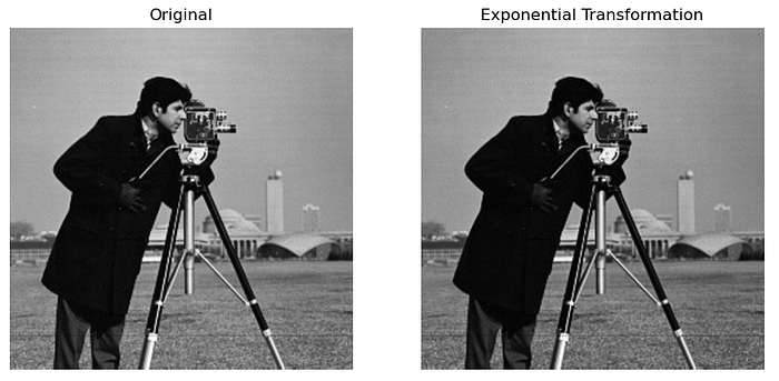
When we want to increase the details in the bright regions and decrease the details in the dark regions of the image, we can use exponential transform, which is the inverse of the logarithmic transform. It’s formula is given in Equation (3):

Equation (3)

Where c is a scaling factor, s is the output pixel and r is the actual pixel. The α is known as base and used to control the compression of the dynamic range(or detail decreasing) in dark regions. As we increase the α, we would expect a better compression. It’s gradient can be depicted as in the Figure (2):

Figure 2

Implementation:

Results:

6.3.Power-law(gamma) Transformation

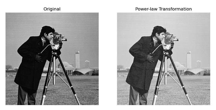
Power-law(gamma) transformation is similiar to both exponential transform and logarithmic transform. The power-law transformation can be expressed as in the Equation (4):

Equation (4)

Where c is a scaling factor, s is the output pixel and r is the actual pixel. For
γ>1, we obtain a result akin to the exponential transform and for γ<1 we can expect a result as we obtained using logarithmic transform. Thus, we can see a gradient like in the Figure 3.

Figure 3

Implementation:

Results:

7.Histogram Sliding

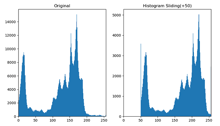
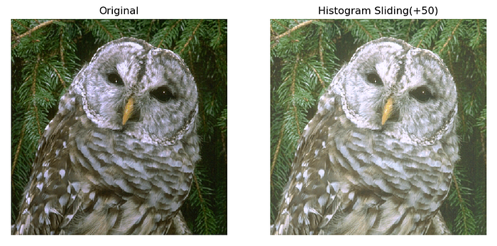
Histogram sliding is one of the most simple contrast enhancement techniques, it basically adds or subtracts a constant intensity value from each pixel while taking care of overflow, with respect to the brightness of the image. If our image is too bright(like washed), we can slide the histogram to the left. If it is too dark, we can slide the histogram to the right. As you can see, we simply increase or decrease the brightness of the image. Histogram sliding can be defined as a piecewise function as in the Equation (5):

Equation (5)

where x is the value of the input pixel, v is the value(negative or positive) used for the histogram sliding, L-1 is the maximum intensity value for an image with L levels.

Implementation:

Results:

The results after running the program above for gray and RGB images:

8.Contrast(Histogram) Stretching

We can use contrast stretching to stretch our intensity values to cover the desired range. This is important for the images whose histogram is narrowed down to a specific range. It is a straight-forward approach as compared to the histogram equalization as well as it is very effective on the images with very low brightness. The transformation can be defined as in the Equation (6):

Equation (6)

In the Equation (6), s is the processed pixel, r is the actual pixel, a is the lowest intensity value and b is the highest intensity value for an image according to bit representation. For a 8-bit image, a and b are respectively 0 and 255. Moreover, c is the lowest intensity value and d is the highest intensity value exists in the image. So the image is normalized. There are different methods for determining c and d, which we will not cover in this article.

Implementation:

Results:

9.Histogram Equalization

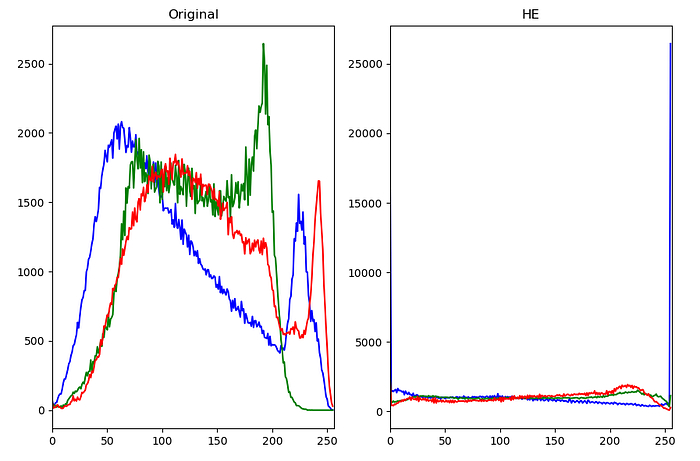
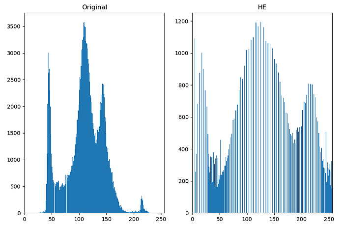
Histogram equalization is more complicated than the methods explained in this article. It’ s aim is to uniformly distribute intensity values over the histogram in order to obtain a flat-like histogram for the image. There are various methods proposed by the researchers in this field. In this section, we will discuss some global approaches to histogram equalization. There are also local methods such as CLAHE and SWAHE. Also, there exist recursive methods such as RMSHE. We may cover and implement these algorithms in our future articles.

9.1. The Classical Histogram Equalization

The classical histogram equalization simply takes an image for equalizing it’s histogram. First of all, assume that we have an input image with L levels, X, with the pixels x(i, j) where i and j are the spatial coordinates of pixel x. We have to find probability of each intensity level in the image. If we divide the number of pixels represents the specific intensity level k by total number of pixels, we can achieve this by using the Equation (7):

Equation (7)

This is called probability density function(pdf). M X N is the total number of pixels, where M is the number of rows and N is the number of columns. The nₖ is the number of pixels belong to the intensity level “k”. We apply this formula for all of the intensity levels and keep them in an array or list. After we have obtained the pdf, now we can calculate the cumulative probability or cumulative distribution function(cdf) with the Equation (8):

Equation (8)

Now, finally, in the last step, we can redistribute the intensities using the transformation function given in Equation (9):

Equation (9)

where X(L-1) is the maximum intensity value.

The algorithm of HE:

1.Calculate probability for each intensity level and obtain pdf starting from 0 to L-1 using Eq. (7)
2.Calculate cdf using Eq. (8)
3.Change the intensity values of the input image with the new intensity values obtained using Eq. (9)
4.Obtain output image

Implementation:

Results:

9.2. Brightness Preserving Bi-histogram Equalization (BBHE)

The Brightness Preserving Bi-histogram Equalization(BBHE) was proposed in [1]. BBHE uses pdf, cdf and transformation functions , however, it divides the image into two parts based on it’s mean. It evaluates these parts individually. The aim of this technique is to preserve overall brightness and reduce the absolute mean brightness error(AMBE). This absolutely provides a better quality histogram equalization. The mean(μ) of the image is the average of the intensity values of all pixels.

Illustration of the BBHE method

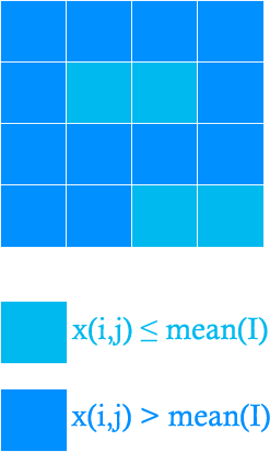
The pixels with the intensity value that is greater than the mean of the image comprises upper part while the rest comprises the lower part. Since we have two parts, we have to calculate the pdf for each of them. We can keep a hashmap to locate these pixels. The pdf calculation for the lower part can be given as in Equation (10):

Equation (10)

The nₖ is the number of pixels belong to the intensity level “k” . Nₗ is the number of pixels in the lower part. Whereas the pdf calculation for upper part can be done with the Equation (11):

Equation (11)

The nₖ is the number of pixels belong to the intensity level “k”. Nᵤ is the number of pixels in the upper part. Now we can calculate cdf for lower and upper parts. For the lower part, we can write the Equation (12):

Equation (12)

Also, for the upper part, we can write the Equation (13):

Equation (13)

Transformations are applied separately on the lower and upper parts, hence, they have to be different. We can define the transformation function for lower part as in the Equation (14):

Equation (14)

Now we can define the transformation function for upper part as in the Equation (15):

Equation (15)

The algorithm of BBHE:

1.Divide the image into lower and upper parts based on the mean
2.Keep the locations of the pixels belong to lower and upper parts in hashmap(s)
3.Calculate cdf and pdf for both of the two parts
4.Apply the appropriate transformation function by looking at the values at hashmaps
5.Obtain output image

Implementation:

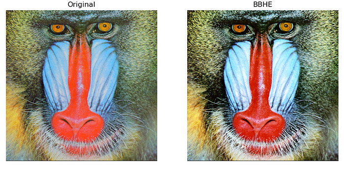
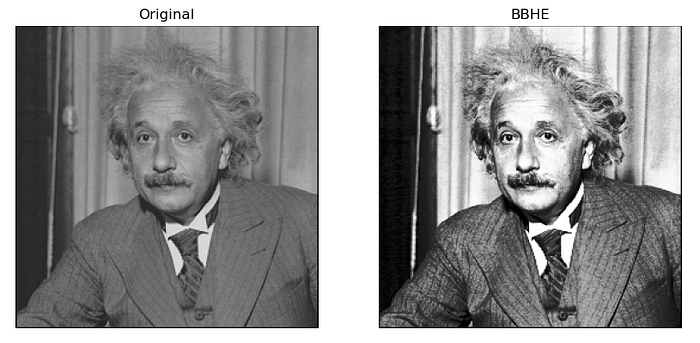
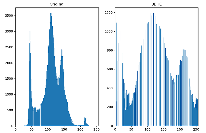
Results:

9.3. Equal Area Dualistic Sub-Image Histogram Equalization (DSIHE)

The Equal Area Dualistic Sub-Image Histogram Equalization(DSIHE) is proposed in [2]. It is similar to the BBHE but it divides the input image depending on the median value. Like classical HE, it calculates the pdf and cdf by using Eq. (7) and Eq. (8) respectively. Then, for each level, it chooses the appropriate threshold to divide the image into two parts according to median, M, using Equation (16):

Equation (16)

The pdf for the lower part can be calculated using Equation (17):

Equation (17)

The pdf for the upper part can be calculated using Equation (18):

Equation (18)

The cdf of the lower part can be given as in Equation (19):

Equation (19)

The cdf of the upper part can be given as in Equation (19):

Equation (20)

We can define the transformation function for lower part as in the Equation (21):

Equation (21)

We can define the transformation function for the upper part as in the Equation (22):

Equation (22)

Illustration of the DSIHE method

The algorithm of DSIHE:

1.Calculate the pdf and cdf of the input image using Eq. (7) and Eq.(8) respectively
2.Using Eq. (16) find the median of the image and divide the image into lower and upper parts
3.Keep the locations of the pixels belong to lower and upper parts in hashmap(s)
3.Calculate cdf and pdf for both of the two parts
4.Apply the appropriate transformation function by looking at the values at hashmaps
5.Obtain output image

Implementation:

Results:

10.Further

You can follow me for more updates. Feel free to contact me if you have any additional question.

E-mail:

emrecankuran21@gmail.com

LinkedIn:

https://www.linkedin.com/in/emre-can-kuran-8470b01b0/

11.References

[1] Yeong-Taeg Kim, “Contrast enhancement using brightness preserving bi-histogram equalization,” in IEEE Transactions on Consumer Electronics, vol. 43, no. 1, pp. 1–8, Feb. 1997, doi: 10.1109/30.580378.

[2]Wang Y, Chen Q, and Zhang B, “Image Enhancement Based On Equal Area Dualistic Sub-Image Histogram Equalization Method”, Consumer Electronics, IEEE Transactions on, (1999), vol. 45, no. 1, pp. 68–75.